Last updated on February 5th, 2025 at 12:36 am
Here, We see Microsoft Excel LinkedIn Skill Assessment Answer. This assessment test consists of 15-20 MCQs to demonstrate your knowledge of your selected skills. MCQs come from different topics – Analysis, Data Manipulation, Formulas, and Setup..
List of all LinkedIn Skills Assessment Answer

Microsoft Excel LinkedIn Skill Assessment Answer
Q1. Some of your data in Column C is displaying as hashtags (#) because the column is too narrow. How can you widen Column C just enough to show all the data?
- Right-click column C, select Format Cells and then select Best-Fit.
- Right-click column C and select Best-Fit.
- Double-click column C.
- Double-click the vertical boundary between columns C and D.✔
Q2. Which two functions check for the presence of numerical or nonnumerical characters in cells?
- ISNUMBER and ISTEXT✔
- ISNUMBER and ISALPHA
- ISVALUE AND ISNUMBER
- ISVALUE and ISTEXT
Q3. If you drag the fill handle (lower-right corner) of cell A2 downward into cells A3, A4, and A5, what contents will appear in those cells?
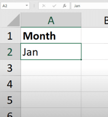
- Jan, Jan, Jan
- Feb, Mar, blank cell
- Feb, Mar, Apr✔
- FEB, MAB, APR
Q4. If cell A3 contains the text THE DEATH OF CHIVALRY, what will the function =PROPER(A3) return?
- the death of chivalry
- The Death of Chivalry
- THE DEATH OF CHIVALRY
- The Death Of Chivalry✔
Q5. In the worksheet below, you want to use Data > Subtotal to show a subtotal value per sport. What must you do BEFORE applying the Subtotal function?
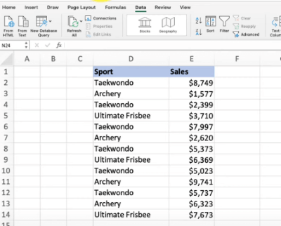
- Sort by the data in Column E.
- Format the data in Column D.
- Sort by the data in Column D.✔
- Format the data in Column E.
Q6. When editing a cell, what do you press to cycle between relative, mixed, and absolute cell references?
- Alt+F4 (Windows) or Option+F4 (Mac)
- Alt+Shift+4 (Windows) or Option+Shift+4 (Mac)
- Ctrl+Shift+4 (Windows) or Command+Shift+4 (Mac)
- the F4 (Windows) or Command+T (Mac)✔
Q7. You need to add a line chart showing sales trends over the last 12 months and you have only a little space to work with. How can you convey the required information within a single cell?
- Add an image of the chart to a comment.
- Add a hyperlink to another worksheet that displays a chart when clicked.
- Add an image of the chart to the worksheet.
- Add a sparkline, a graphic that summarizes data visually within a single worksheet cell.✔
Q8. What is the best way to activate the Excel Help system?
- Right-click anywhere and select Help.
- Press F1 or click the Help tab in the ribbon.✔
- Press F10.
- all of these answers.
Q9. Which format will display the value 27,500,000 as 27.5?
- ##,###,,
- ###.0,,✔
- 999.9,,
- ###,###.0,
Q10. When using Goal Seek, you can find a target result by varying _ at most.
- three inputs
- four inputs
- two inputs
- one input✔
Q11. In the image below, which option(s) can you select so that the appropriate field headers appear in cells A4 and B3 instead of the terms Row Labels and Column Labels, respectively?

- Show in Tabular Form
- Show in Compact Form
- Show in Compact For or Show in Outline Form
- Show in Tabular Form or Show in Outline Form✔
Q12. Which formula is NOT equivalent to all of the others?
- =A3+A4+A5+A6
- =SUM(A3:A6)
- =SUM(A3,A6)✔
- =SUM(A3,A4,A5,A6)
Q13. What custom formatting can be applied to make the cells in column A resemble the cells in column B?
- MMM-YYYY
- MMMM-YYYY✔
- MMMM&”-“&YYYY
- M-YYYY
Q14. Which function returns a reference to a cell (or cell range) that is a specified distance from a base cell?
- OFFSET✔
- VLOOKUP
- INDEX
- MATCH
Q15. You’re working with columns whose width and font size should not be changed. Yet the columns are too narrow to display all the text in each cell. What tool should you use to solve the problem?
- Sparklines
- Wrap Text✔
- Fill Handle
- Centered Alignment
Q16. Of the four chart types listed, which works best for summarizing time-based data?
- pie chart
- line chart✔
- XY scatter chart
- bar chart
Q17. The AutoSum formulas in the range C9:F9 below return unexpected values. Why is this?

- The AutoSum formulas refer to the column to the left of their cells.
- The AutoSum formulas exclude the bottom row of data.
- The AutoSum formulas include the year at the top of each column in the calculation. The formula bar clearly shows it’s the dates (top row) included, along with the total (bottom) row. Thus, the bottom row of data is not excluded.✔
- The AutoSum formulas include their own cells, creating a circular reference.
Q18. The text filter in column A is designed to display only those rows where the column A entry has a particular attribute. What is this attribute?

- The second character in the cell is 9.✔
- The number 9 appears one or more times within the cell.
- The cell is comprised of 9 characters.
- The number 9 appears once and only once within the cell.
Q19. An organization chart, which shows the hierarchy within a company or organization, is available as _ that is included with Excel.
- a 3D model
- SmartArt✔
- a Treemap chart
- a drawing object
Q20. You want to be able to restrict values allowed in a cell and need to create a drop-down list of values from which users can choose. Which feature should you use?
- Protect Worksheet
- Conditional Formatting
- Allow Users to Edit Ranges
- Data Validation✔
Q21. To round up a value to the nearest increment of your choice, such as the next five cents, what function should you use?
- ROUNDUP✔
- MAX
- ROUND
- CEILING
Q22. Which function returns the largest value amongst all values within the range H2:H30?
- =MAX(H2:H30)✔
- =MAXIMUM(H2:H30)
- =LARGE(H2:H30,29)
- =UPPER(H2:H30,1)
Q23. Which chart type can display two different data series as a different series type within the same chart?

- XY chart
- clustered column
- bubble chart
- combo chart✔
Q24. In the image below, what does clicking the button indicated by the green arrow do?

- Hides or shows the formula bar.
- Selects all.✔
- Hides or shows the ribbon.
- Selects objects.
Q25. Which formula returns the value in cell A1 of the worksheet named MySheet?
- =MySheet!A1✔
- =MySheet_A1
- =MySheet&A1
- =MySheet@A1
Q26. In the worksheet below, you want to copy the formatting of cell A1 into cells B1:D1. Which approach (see arrows) accomplishes this the most efficiently?
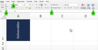
- B
- C
- A✔
- D
Q27. Which formula correctly counts the number of numeric values in both B4:E4 and G4:I4?
- =COUNT(B4:E4&G4:I4)
- =COUNT(B4:E4,G4:I4)✔
- =COUNT(B4:E4 G4:I4)
- =COUNT(B4:I4)
Q28. After activating a chart, which sequence adds a trendline to the chart?
- In the Format group, select Trendline from the Insert Shapes list.
- Click outside the plot area and select Add Trendline
- Click inside the plot and select Forecast.
- Right-click a data series and select Add Trendline.✔
Q29. Which Excel add-in will help you find a target result by varying multiple inputs to a formula?
- Goal Seek✔
- Power Pivot
- Data Analysis
- Solver
Q30. What tool would you use to prevent the input in a cell of a date outside a specific range?
- Protect Workbook
- Watch Window
- Data Validation✔
- Filter
Q31. When you sort a list of numerical values into ascending or descending order, the value in the middle of the list is the _.
- mode
- modulus
- average
- median✔
Q32. Which format setting does not change the background appearance of a cell?
- Cell style
- Fill color
- Pattern style
- Font color✔
Q33. In Excel, what do most formulas begin with?
- :
- =✔
- (
- –
Q34. You need to determine the commission earned by each Sales Rep, based on the Sales amounts in B3:B50 and the Commission rate specified in cell A1. You want to enter a formula in C3 and copy it down to C50. Which formula should you use?
| A | B | C | |
|---|---|---|---|
| 1 | 8.5% | 2018 Commission | |
| 2 | Sales Rep | 2018 Sales | Commission Earned |
| 3 | Jordan Hinton | $123,938.00 | |
| 4 | Lilah Douglas | $5594,810.00 | |
| 5 | Karyn Reese | $235,954.00 | |
| 6 | Chiquita Walsh | $684,760.00 |
- =$A1*B3
- =$A$1*B3✔
- =A1*$B3
- =A1*B3
Q35. If you start a date series by dragging down the fill handle of a single cell that contains the date 12/1/19, what will you get?
- a series of consecutive days following the initial date✔
- a series of days exactly one month apart
- a series of days identical to the initial date
- a series of days exactly one year apart
Q36. To discover how many cells in a range contain values that meet a single criterion, use the _ function.
- COUNT
- SUMIFS
- COUNTA
- COUNTIF✔
Q37. Your worksheet has the value 27 in cell B3. What value is returned by the function =MOD (B3,6)?
- 4
- 1
- 5
- 3✔
Q38. For an IF function to check whether cell B3 contains a value between 15 and 20 inclusively, what condition should you use?
- OR(B3=>15,B3<=20)
- AND (B3>=15,B3<=20)✔
- OR(B3>15,B3<20)
- AND(B3>15, B3<20)
Q39. The charts below are based on the data in cells A3:G5. The chart on the right was created by copying the one on the left. Which ribbon button was clicked to change the layout of the chart on the right?
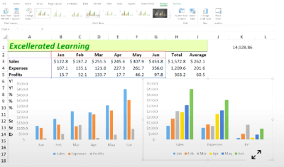
- Move Chart
- Switch Row/Column
- Quick Layout
- Change Chart Type✔
Q40. Cell A20 displays an orange background when its value is 5. Changing the value to 6 changes the background color to green. What type of formatting is applied to cell A20?
- Value Formatting
- Cell Style Formatting
- Conditional Formatting✔
- Tabular format
Q41. What does this formula do? =Sum(Sheet1:Sheet4!D18)
- It adds data from cell D18 of Sheet1 and cell D18 of Sheet4
- It adds data from cell A1 of Sheet1 and cell D18 of sheet4
- It adds all data in the range A1:D18 in Sheet1, Sheet2, Sheet3 and Sheet4
- It adds data from all D18 cells in Sheet1, Sheet2, Sheet3 and Sheet4✔
Q42. What is the term for an expression that is entered into a worksheet cell and begins with an equal sign?
- function
- argument
- formula✔
- contents
Q43. How does the appearance of an array formula differ from that of a standard formula?
- In a worksheet cell, array formulas have a small blue triangle in the cell’s upper-right corner.
- A heavy border appears around the range that is occupied by the array formula.
- In the formula bar, an array formula appears surrounded by curly brackets.✔
- When a cell that contains an array formula is selected, range finders appear on the worksheet around the formula’s precedent cells.
Q44. In a worksheet, column A contains employee last names, column B contains their middle initials (if any), and column C contains their first names. Which tool can combine the last names, initials, and first names in column D without using a worksheet formula?
- Concatenation✔
- Columns to Text
- Flash Fill
- AutoFill
Q45. Which formula returns the value in cell A10 of the worksheet named Budget Variances?
- =’Budget Variances’!A10✔
- =’Budget Variances!A10′
- =”BudgetVariances!A10″
- =”BudgetVariances”!A10
Q46. Which function returns the leftmost five characters in cell A1?
- =FIND(A1,1,5)
- =SEARCH(A1,5)
- =LEFT(A1,5)✔
- =A1-RIGHT(A1,LEN(A1)-5)
Q47. Which function returns TRUE if cell A1 contains a text value?
- =ISALPHA(A1)
- =ISCHAR(A1)
- =ISSTRING(A1)
- =ISTEXT(A1)✔
Q48. You select cell A1, hover the pointer over the cell border to reveal the move icon, and then drag the cell to a new location. Which ribbon commands achieve the same result?
- Cut and Fill
- Cut and Paste✔
- Copy and Transpose
- Copy and Paste
Q49. You want to add a column to the Pivot Table below that shows a 5% bonus for each sales rep. That data does not exist in the original data table. How can you do this without adding more data to the table?
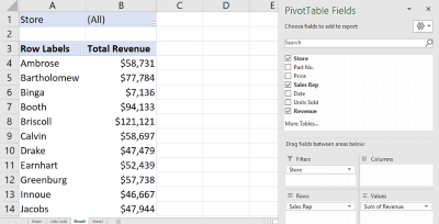
- Add a new PivotTable field.
- Add a calculated item
- Add a new Summarize Value By field.
- Add a calculated field.✔
Q50. You need to determine the commission earned by each Sales rep, based on the Sales amount in B3:B50 and the Commission rate specified in cell A1. You want to enter a formula in C3 and copy it down to C50. Which formula should you use?
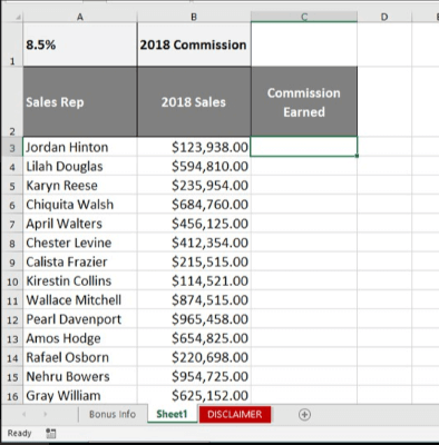
- =A1*$B3
- =A1*B3
- =$A$1*B3✔
- =$A1*B3
Q51. The NOW() function returns the current date and time as 43740.665218. Which part of this value indicates the time?
- 6652
- 43740.665218
- 43740
- 665218✔
Q52. Cell A2 contains the value 8 and cell B2 contains the value 9. What happens when cells A2 and B2 are merged and then unmerged?
- Both values are lost.
- Cell A2 contains the value 8 and cell B2 is empty.✔
- Cell A2 contains the value 8 and cell B2 contains the value 9.
- Cell A2 contains the value 17 and cell B2 is empty.
Q53. In the formula =VLOOKUP(A1,D1:H30,3,FALSE), the lookup value (A1) is being looked for in _.
- column D✔
- columns D through H
- column H
- column F
Q54. An .xlsx workbook is saved in .csv format. What is preserved in the new .csv file?
- cell values only✔
- cell values and formats
- cell values and formulas
- cell value, formats, and formulas
Q55. Which function, when entered into cell G7, allows you to determine the sum total of annual sales for market regions 18 and greater?
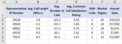
-
=SUMIF(G2:G6,">17",F2:F6) - =SUM(G2:G6,”>=18,F2:F6)
- =SUMIF(F2:F6,”>=18″,G2:G6)✔
- =SUM(F2:F6,”18+”,G2:G6)
Q56. Which function, when entered into cell F2 and then dragged to cell F6, returns the performance rating text (e.g., “Good”, “Poor”) for each representative?

- =RIGHT(E2,LEN(E2)-27)✔
- =LEN(E2,MID(E2)-27)
- =LEFT(E2,LEN(E2)-27)
- =RIGHT(E2,MID(E2)-27)
Q57. What is Colors[Inventory] referring to here?
=SUMIFS(Colors[Inventory],Colors[Colors],"Orange")- The inventory worksheet in the Colors workbook
- the Inventory column in the Colors table✔
- the Colors worksheet in the Inventory workbook
- the named range Colors[Inventory], which does not use Format as Table Feature
Table[Column] can be used instead of cell references (C2:C7). Reference
Q58. Which VLOOKUP function, when entered into cell L2 and then dragged to cell L5, returns the average number of calls for the representative IDs listed in column J?
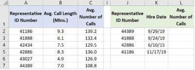
- =VLOOKUP(A2,J2:L5,1,FALSE)
- =VLOOKUP(J2,A$2:C$7,1,FALSE)
- =VLOOKUP(J2,A$2:C$7,3,FALSE)✔
- =VLOOKUP(J2,A2:C7,3,FALSE)
Q59. Which formula calculates the total value of a single row of cells across a range of columns?
- =SUBTOTAL(C1:Y15)
- =SUM(15L:15Z)
- =SUM(C15:Y15)✔
- =SUM(C11:C35)
The sum of columns C to Y for the same row 15.
Q60. Which value is returned when you enter =LEN(C3) into cell F3?

- 4
- 5✔
- 3
- 2
Q61. How can you create the lower table from the top one when the tables are not linked?
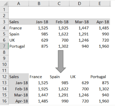
- Select Paste Special > Values.
- Select Paste Special > Transpose.✔
- Use the TRANSPOSE function
- Click Switch Rows & Columns
Because it needs to be transposed without creating a reference.
Q62. Which function returns the number of characters in a text string in cell A1?
- =RIGHT(A1)-LEFT(A1)+1
- =LEN(A1)✔
- =EXACT(A1)
- =CHARS(A1)
Q63. Which formula, when entered into cell D2 and then dragged to cell D6, calculates the average total number of minutes spent on phone calls for each representative?
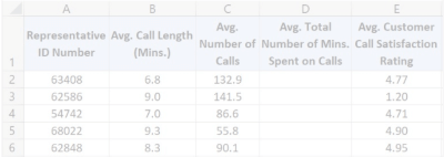
- =B$2*C$2
- =$C$2/$B$2
- =C2/B2
- =B2*C2✔
Q64. The Pivot Table below has one-row field and two column fields. How can you pivot this table to show the column fields as subtotals of each value in the row field?
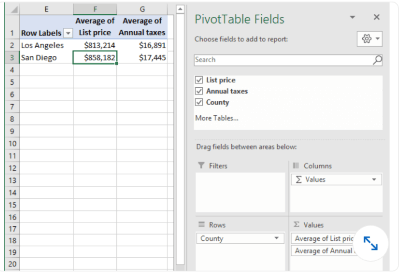
- On the PivotTable itself, drag each
Averagefield into the row fields area. - Right-click a cell in the PivotTable and select PivotTable Options > Classic PivotTable layout.
- In the PivotTable Fields pane, drag Sum Values from the Columns section to a location below the field in the Rows section.✔
- In the
PivotTable Fieldspane, drag each field from theSum Valuessection to theRowssection.
Q65. Which Excel feature allows you to hide rows or columns with an easily visible expand/collapse?
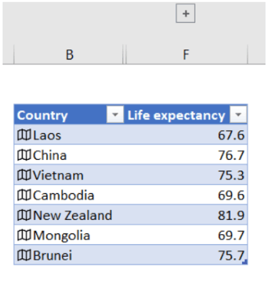
- grouping✔
- filtering
- hiding
- cut and paste
Q66. Monthly revenues of 2019 are entered in B2:M2, as shown below, To get year-to-date running total revenues, what formula should you enter in B3 and autofill through M3?

- =SUMIF($B$2:$M$2,”COLUMN($B$2:$M$2)<=COLUMN())”)
- =SUM($B2:B2)✔
- =SUM(OFFSET($A1,0,0,1,COLUMN()))
- =B2+B3
We are calculating the running total here.
Q67. From which field list was the PivotTable created?
(Missing screenshot)
- rows:event, donor/values: Sum of amount
- columns: event / row: donor/values: Sum of amount
- rows:donor, event/values: Sum of amount✔
- filter: event / row: donor/values: Sum of amount
Q68. In the worksheet shown below, cell C6 contains the formula =VLOOKUP(A6,$F$2:$G$10,2,FALSE). What is the most likely reason that #N/A is returned in cell C6 instead of Mallory’s ID (2H54)
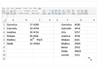
- The absolute/relative cell references in the formula are wrong
- Cell A6 is not actually text it is a formula that needs to be copied and pasted as a value
- Column C in the lookup range is not sorted properly
- A trailing space probably exists in cell A6 or F7✔
Q69. What is the difference between pressing the delete key and using the clear command in the Home tab’s Editing group?
- Deletes remove the entire column or row. Clear removes the content from the column or row
- Deletes remove formulas, values, and hyperlinks. clear remove formulas, values, hyperlinks, formats, comments, and notes✔
- Delete removes the cell itself, shifting cells either up or to the left. Clear removes content and properties but does not move cells
- Delete removes formulas and values. clear remove formulas, values, hyperlinks, formats, comments, and notes
Q70. What is the intersection of a worksheet row and column?
- Cell✔
- Selection
- Element
- Scalar
Q71. In this Pivot Table, the continuous variable weight is shown in the Row field. Another continuous variable is in the Sum Values field. It is important to reduce a long list of body weights to a smaller set of weight categories. How do you do this?
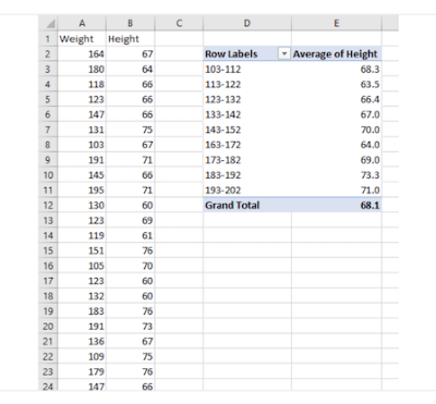
- Use weight as a filter field as well as a row field in the Pivot Table.
- Use
IF()to show weight by categories instead of by pounds. - Click the Row Labels arrow and select Group.
- Right-click any row field value in the PivotTable and select Group.✔
Q72. How can you drill down into a Pivot Table to show details?
- Select the cell into which you want to drill down, right-click, and select Show Summary.
- Select the cell into which you want to drill down, right-click and select Drill-down.
- Select the cell into which you want to drill down and double-click.✔
- Select the cell into which you want to drill down, right-click, and select Show Details > Summary Page
Q73. To ensure the VLOOKUP function returns the value of an exact match, what do you need to enter into the Range_lookup field?

- 0
- 1
- FALSE✔
- TRUE
Q74. Cell D2 contains the formula =B2-C2. What is the fastest way to copy that formula into cells D3:D501 (the bottom of the data set)?
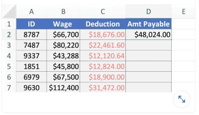
- Right-click D2 and select Fill Down.
- Click D2’s fill handle and drag it down to D501.
- On the ribbon’s Data tab, select Flash Fill.
- Double-click D2’s fill handle.✔
Q75. This data needs to be sorted by Group, then by Last Name, then by First Name. How do you accomplish this?
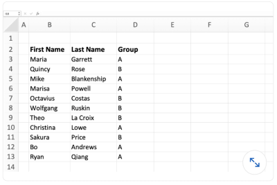
- A
- Rearrange the columns in this order: Group, Last Name, First Name.
- Right-click any of the headers.
- Select Sort All.
- B
- Select any cell in the dataset.
- In the Data tab, click the Sort button.
- Add two levels to the default level.
- Populate the Sort-by fields in this order: Group, Last Name, First Name.
- C✔
- Highlight the entire dataset.
- In the Data tab, click the Sort button. The headers appear.
- Drag the headers into this order: Group, Last Name, First Name.
- D
- Select a cell in the Group column, then sort.
- Select a cell in the Last Name column, then sort.
- Select a cell in the First Name column, then sort.
Q76. How can you use Format Painter to apply the format of a single source cell to several nonadjacent destination cells?
- A
- Right-click the source cell.
- Click the Format Painter.
- Right-click each destination cell.
- Press Esc.
- B
- Ctrl-click (Windows) or Command-click (Mac) each destination cell to select it.
- Click the Format Painter.
- Click the source cell.
- C✔
- Select the source cell.
- Double-click the Format Painter.
- Click each destination cell.
- Press Esc.
- D
- Select the source cell.
- Right-click the Format Painter.
- Click each destination cell.
- Press Esc.
Q77. Which is a valid Excel formula?
- =(A5+B5)*B7✔
- =A3-7(B3:B5+4)
- =(A5+B5)B7
- =B3^[2*/3]
Q78. Columns D, E, and F are hidden in your worksheet. What is one way to unhide these columns?
- Select column G, then right-click and select Unhide.
- Select column C, then right-click and select Unhide.
- On the Page Layout tab, in the
RowsandColumnssection, select Unhide. - Click and drag to select columns C and G, then right-click and select Unhide.✔
Q79. Before publishing a document, you want to identify issues that may make it difficult for people with disabilities to read. Which feature should you use?
- Check Accessibility✔
- Check Compatibility
- Protect Document
- Inspect Document
Q80. How do you remove the background of an inserted image?
- Select the image and, on the Picture Tools Format tab, use the
Compress Picturefeature. - Select the image and, on the
Designtab, use the Format Background feature. - On the Drawing Tools Format tab, select
Graphics Fill>Remove Background. - Select the image and, on the Picture Tools Format tab, click the Remove Background button.✔
Q81. What is the result of the formula =4&3?
- 43✔
- 12
-
#VALUE! - 7
Q82. How do you remove everything (values, formatting, etc.) from a cell?
- Select the cell. On the Home tab, click Clear.
- Select the cell and press Delete.
- Right-click the cell and select Delete.
- Select the cell. On the Home tab, click Clear > Clear All.✔
Q83. What is the difference between a workbook and a worksheet?
- An Excel file is a workbook. A workbook contains one or more worksheets.✔
- Nothing-these two terms mean the same thing.
- A workbook contains only data. A worksheet contains both data and formulas.
- An Excel file is a worksheet. A worksheet contains one or more workbooks.
Q84. How would you connect the slicer to both PivotTables?

- You cannot use one slicer for two PivotTables.
- Right-click the slicer and select Slicer Settings.
- Merge the two PivotTables, right-click the merged PivotTable, and select Combine Slicer.
- Right-click the slicer and select Report Connections, or click Report Connections on the Slicer tab.✔
Q85. Which formula contains a valid absolute reference?
- =B7*$G$3✔
- =(B7)*G3
- =B7*$[G3]
- =B7$*G3
Q86. What happens if you use the AutoSum button in cell H4?
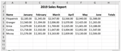
- AutoSum shows the total in the bottom-right of the page
- AutoSum will total the numbers in cells B4:G8
- AutoSum will total the numbers in cells B4:G4✔
- AutoSum will return a #VALUE! error.
Q87. To create this PivotTable, drag the _ field to the Rows area and the _ field to the Values area.
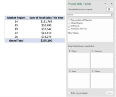
- Total Sales This Year; Total Sales This Year
- Total Sales This Year; Market Region
- Representative ID Number; Total Sales This Year
- Market Region; Total Sales This Year✔
Q88. Cell A1 contains the number 3. Which formula returns the text Apple?
- =SELECT(A1, “Banana”, “Orange”, “Apple”, “Mango”)
- =CHOOSE(A1, “Banana”, “Orange”, “Apple”, “Mango”)✔
- =CHOOSE(A1,”Banana”,”Orange”,”Apple”,”Mango”)✔
- =MATCH(A1,{“Banana”,”Orange”,”Apple”,”Mango”})
Q89. Which value is calculated when the formula =AVERAGE(G2:G6)/AVERAGE(C2:C6) is entered into cell H7?

- average number of minutes per call
- average annual sales per minute
- average number sales
- average annual sales per call✔
Q90. How would you search an entire workbook with Find & Select?
- On the Home tab, click Find & Select > Find > Options (Windows) or Find & Select > Find (Mac). Change the Within drop-down to Workbook.✔
- On the Home tab, click Find & Select > Find > Options (Windows) or Find & Select > Find (Mac). Change the Look in drop-down to Workbook.
- On the Home tab, click Find & Select > Find > Options (Windows) or Find & Select > Find (Mac). Change the Search drop-down to All.
- You cannot search an entire workbook – you must search the worksheets individually.
Q91. How do you create a heatmap in a table, such as this one, which is responsive to the values?

- map chart
- color scales (within conditional formatting)✔
- Manual highlighting
- data bars (within conditional formatting)
Q92. To split text across cells without using Merge & Center, click Format Cells. Then, on the Alignment tab, click_.
- Text control > Merge cells✔
- Horizontal > Center across selection
- Vertical > Center across selection
- Data tab > Text to columns
Q93. In the worksheet below, what do the symbols in rows 4, 6, 7, and 11 indicate?
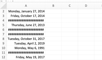
- The dates are erroneous, such as October 39, 2015.
- The columns aren’t wide enough to show the full date.✔
- The times are incorrectly formatted as dates.
- The text is incorrectly formatted as dates.
Q94. You are determining % growth by dividing Growth by Sales. Which Excel function would you use to avoid #DIV/0! errors?
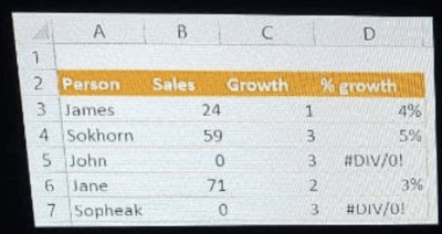
- IFERROR✔
- ROUND
- ISERROR
- DIVIDE
Q95. You have a worksheet in Excel that will print as 10 pages. How can you ensure that the header row is printed at the top of each page?
- Use Print Titles on the Page Layout tab.✔
- Use Page Setup from the Backstage View.
- Use Freeze Panes on the View tab.
- Format your data as a table; the header prints automatically.
Q96. Which value is returned when you enter this function into cell G2? =IF(SUM(F2:F6)>12,”Too Many Tardy Days”,”No Tardiness Issue”)

- Too Many Tardy Days
- #NUM!
- No Tardiness Issue✔
- #REF!
Q97. What ribbon command on the Home tab can you use to change a cell’s fill color automatically, based on the value of the cell?
- Conditional Formatting✔
- Format
- Cell Styles
- Fill
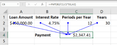
Q98. In this worksheet, how are cells A2:D2 related to cell C4?
- Cells A2:D2 are comments relating to the formula in cell C4.
- Cells A2:D2 are the source of an error in the formula in cell C4.
- Cells A2:D2 are precedents of the formula in cell C4.✔
- Cells A2:D2 are dependent on the formula in cell C4.
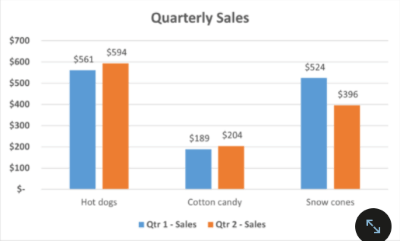
Q99. What is the name given to the numbers in or above each bar in a column chart, as shown?
- data table
- data numbers
- data labels✔
- data values
Q100. Which chart type provides the best visual display of the relationship between two numeric variables?
- radar chart
- box and whisker chart
- XY scatter chart✔
- combo chart
Q101. To ensure that a collection of shapes is evenly spaced apart from left to right, select the shapes, click Page Layout > Align, and then click _.
- Distribute Horizontally✔
- Align Center
- Distribute Vertically
- Align Middle
Q102. A file extension of .xlsm indicates what type of workbook?
- macro-enabled workbook✔
- XML-standard workbook
- Excel 2003 workbook
- workbook where macros are not allowed
Q103. How do you remove only the conditional formatting from a cell and leave all other formatting intact?
- This is not possible you can remove only all formatting from a cell.
- Select the cell. On the Home tab, click Conditional Formatting > Clear Rules > Clear Rules from Selected Cells.✔
- Right-click the cell and select Delete Conditional Formatting.
- Right-click the cell and select Remove Conditional Formatting.
Q104. If a range name is used in a formula and the name is deleted, what happens to the formula?
- The formula displays a warning but the actual cell address is substituted for the deleted name.
- The formula becomes invalid and displays a #NAME? error.✔
- The actual cell addresses replace the original range name in the formula.
- The formula becomes invalid and displays a #N/A error
Q105. You want to restrict the values entered in a cell to a specified set, such as Hop, Skip, or Jump. Which type of data validation should you use?
- input range
- list✔
- custom
- database
Q106. You want to find the second-largest invoice in a column containing all the invoices in a given month. What function would you use?
- NEXT
- MAX
- LARGE✔
- MATCH
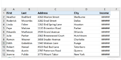
Q107. How can you see the data in column E?
- Close the workbook without saving it and reopen it.
- Turn off conditional formatting.
- On the Home tab of the ribbon, select Fit to Column.✔
- Expand the width of its column.
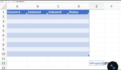
Q108. In the worksheet below, a table called Projects extends from cell A1 to D10. Cell D1 contains the text Status. Cell E12 contains the formula =Projects[@Status]. What does this formula return?
- #VALUE!
- a blank cell
- #REF!✔
- 0
Q109. Which Excel feature allows you to select all cells in the column with inconsistent formulas compared to the rest of the column?

- On the Home tab, click Go To > Special > Column differences.✔
- On the Formulas tab, click Trace precedents.
- On the Formulas tab, click Trace errors.
- On the Formulas tab, click Show Formulas
Q110. What is one way to center text in a cell?
- Right-click the cell and select Center (Windows) or Center Text (Mac).
- Select the cell and, on the View tab in the Cells section, click Alignment and select Center (Windows) or Center Text (Mac).
- Select the cell and, on the Home tab in the Alignment section, click Center (Windows) or Center Text (Mac).✔
- Change the width of the cell until the text is centered.
Q111. Cell D1 contains the value 7.877. You want cell D1 to display this value as 7.9 but keep the original number in calculations. How can you accomplish this?
- Click the Decrease Decimal button once.
- Click the Decrease Decimal button twice.✔
- Use the
ROUND()function. - In the Cells group on the Home tab, click Format > Format Cells. Then click the Alignment tab and select Right Indent.
Q112. Given the image below, what happens if you type “P” in cell A6?
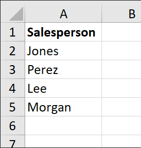
- The word “Perez” appears and immediately the active cell moves down.
- The word “Perez” appears and the active cell remains in Edit mode.✔
- A pop-up list appears with the previous four names.
- The letter “P” appears.
Q113. To insert a new column to the left of a specific column, right-click the header containing the column’s letter and select _.
- Insert Column
- Paste Special
- Insert✔
- Insert Column Left
Q114. Your transactions data set contains more than 10,000 rows. Some rows contain the same transaction. How would you remove the rows containing identical transactions?
- Filter the relevant column, right-click the column head, and select Remove Duplicates.
- This is possible only with Power Query.
- With the data selected, on the Data tab click Remove Duplicates.✔
- This is possible only using formulas.
Q115. A colleague shared an Excel file with you, and you want to display a worksheet that is hidden in it. How you can do that?
- On the Home tab, click Unhide.
- On the Review tab, click Unhide Sheet.
- On the View tab, click New Window.
- Right-click on any worksheet tab and select Unhide✔
Q116. You have a column of dog breeds that are in all capital letters. What function would you use to convert those dog breeds so that only the first letter of each word is capitalized?
- Sentence
- Upper
- Titlecase
- Proper✔
Q117. In cell C2, how would you limit the user to choosing one of the company’s five regions(East, Central, North, South, West)?

- Use reference tabs to create a drop-down list
- Use a PivotTable slicer to create a drop-down list
- Insert a table in the data to create a drop-down list
- Use data validation to create a drop-down list✔
Q118. To calculate gross pay, hours are multiplied by the hourly rate. What formula would you put in cell C4 to then able to copy that cell down to the rest of the column
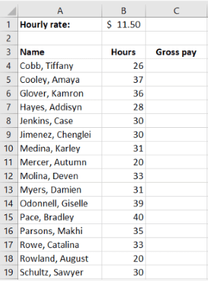
- =B1*$B$4
- =$B1*B4
- =B1*B4
- =$B$1*B4✔
Q119. What do blue row numbers indicate?

- The cells are selected/highlighted
- Excel’s options have been changed
- Certain rows in the data set are hidden
- A filter is applied✔
Q120. Based on the data in columns D, G, H, and K below, what formula will calculate the average compensation for full-time employees who have a job rating of 5?
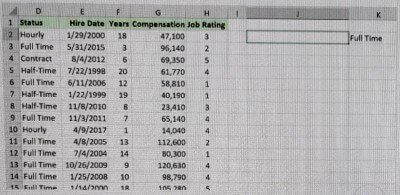
- =AVERAGEIF(D:D,K2,H:H,5,G:G)
- =AVERAGEIF(G:G,D:D,K2,H:H,5)
- =AVERAGEIFS(K2,H:H,5,G:G)
- =AVERAGEIFS(G:G,D:D,K2,H:H,5)✔
Q121. Which feature enables you to quickly sort and reduce data to a subset?
- data validation
- conditional formatting
- advanced sort
- filters✔
Q122. You have a formula in cell A1. You want to display that formula in cell B1. What function can you use in cell B1?
- TEXT
- FORMULATEXT✔
- ISFORMULA
- ISTEXT
Q123. You want to remove the unprintable characters and unnecessary spaces from column A. What formula would you put into cell B2 to copy down to the rest of the column?
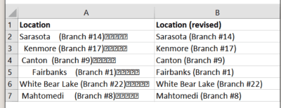
- =ERROR.TYPE(A2)
- =CLEAN(TRIM(A2))✔
- =CHOOSE(A2)
- =TRIM(A2)
Q124. What is the output of the formula =(8+2*3)/7?
- 13
- 2✔
- 11
- 15
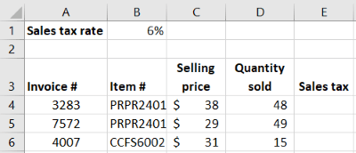
Q125. The amount of sales tax on each sale is calculated as the selling price times the quantity sold times the sales tax rate. What formula would you use in cell E4 to then be able to copy that cell to the rest of the column?
- =C4*D4*$B$1✔
- =(C4*D4)*B1
- =C4*D4*B1
- =C4*D4(*B1)
Q126. Which is not a way to edit a formula in a cell?
- Press F2.
- Select the cell and then click on the formula bar.
- Double-click the cell
- Right-click the cell and select Edit✔
Q127. What does this formula do?
=SUM(Sheet1:Sheet4!D18)
- It adds data form all D18 cells in Sheet1, Sheet2, Sheet3, Sheet4✔
- It adds data from cell D18 of Sheet1 and cell D18 of Sheet4
- It adds all data in the range A1:D18 in Sheet1,Shee2, Shee3, and Sheet4
- It adds data from cell A1 of Sheet1 and cell D18 of Sheet4
Q128. You realize that you named a table Quraters and want to correct it as Quarters. How could you accomplish this?
- On the Table Design tab (Windows) or Table tab (Mac), rename the table in the Table Name box.✔
- Copy the table to another worksheet and rename it Quarters.
- Right-click in the table and select Rename.
- On the Table Design tab (Windows) or Table tab (Mac), click Name Manager.
Q129. Which function is best used to look up and retrieve data from a specific row in a table?
- HLOOKUP
- MATCH
- VLOOKUP✔
- ADDRESS
Q130. When you provide alt text for an image, what type of control are you including?
- password protection
- presentation
- layout
- accessibility✔
Q131. Which tool provides the easiest way to create and insert an organizational chart into a presentation?
- Charts
- 3D Models
- Shapes
- SmartArt✔
Q132. You are creating a slide that shows annual rainfall in different regions of Europe. What chart type would most effectively communicate that relationship?
- line chart
- scatter chart
- pie chart
- map chart✔
Q133. Column A contains a list of book titles. To ensure that no book title appears more than once, first you select column A. What should you do next?
- Right-click the column head and select Unique
- On the Home ribbon, click Clear > Duplicates
- On the Data ribbon, click Remove Duplicates✔
- On the Data ribbon, click Data Validation
Q134. You want to copy only the cells that are displayed here – not the hidden cells – into another worksheet. After selecting the cells in the worksheet, how do you accomplish this?
- On the View tab, select Visible cells only, Paste into the destination worksheet
- On the Home tab, clear the Hidden Cells check box. Paste into the destination worksheet
- Copy the cells. Then in the destination worksheet, click Paste Special> Paste only visible cells
- On the Home tab, click Find & Select > Go to Special> Visible cells only. Paste into the destination worksheet✔
Q135. You want to define a reusable process to reshape data (removing blank rows, merging columns, etc.). What tool can you use to accomplish this?
- Power Query✔
- Data Analysis
- Power Pivot
- Data Modeler
Q136. You want to be able to restrict values allowed in a cell and need to create a drop-down list of values from which users can choose. Which feature should you use?
- Project Worksheet
- Data validation✔
- Conditional Formatting
- Allow Users to Edit Ranges
Q137. Which situation will result in a #REF! error?
- The cell referenced in the error message has been deleted✔
- A non-numeric argument is used in a function when a numeric value is expected
- A required operator is omitted in a formula
- The formula contains an undefined range
Q138. Which feature allows formatting to be automatically added to new columns and rows?
- AutoFormat
- conditional formatting
- Format as Table✔
- PivotTable
Q139. What Excel feature can you use to automatically format cells that are greater than a specified value with designated fill and text colors?
- Flash Fill
- Conditional Formatting✔
- Format as Table
- Theme Colors
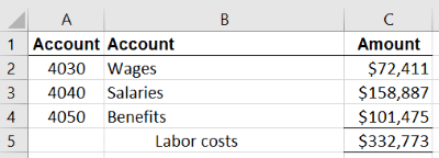
Q140. Which formula could not have been entered in cell C5?
- =SUBTOTAL(9, C2:C4)✔
- =C2+C3+C4
- =SUBTOTAL(C2:C4)
- =SUM(C2:C4)
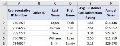
Q141. The last two digits of the Representative ID Number are the Office ID. Which function, when entered into cell B2 and then dragged to cell B6, returns the Office ID for each representative?
- =TRIM(A2,2)
- =LEFT(A2,2)
- =RIGHT(A2,2)✔
- =MID(A2,2)
Q142. What is the fastest way to see the data in column E

- Double-click between column headers E and F✔
- Double-click between column headers F and G
- On the Home tab of the ribbon, select Fit to Column
- Drag to resize the column
Q143. Excel’s default view contains the Quick Access Toolbar and the ribbon. Which can you customize?

- You cannot customize either.
- only the ribbon
- both the Quick Access Toolbar and the ribbon✔
- only the Quick Access Toolbar
Q144. Other than pasting an image, how can you insert an image file from your computer into a worksheet?
- On the Insert tab, click Pictures > This Device (Windows) or Pictures > Picture from file (Mac)✔
- On the Insert tab, click SmartArt > Copy Image from Device (Windows) or SmartArt > Copy (Mac)
- On the Insert tab, click Illustrations > Insert Illustration from This Device
- On the Insert tab, click Icons > Insert > Picture from This Device
Q145. You want to restrict a user from entering any amount greater than $100 or less than $20 in a row. Which Excel feature would you use?
- There is not a feature in Excel that will do this.
- Data Limiting
- Data Parameters✔
- Data Validation
Q146. What is the output of the formula =(8+2*3)/2?
- 13
- 15
- 11
- 7✔
Q147. How many columns are in the Excel sheet by default?
- 16000
- 1,048,576
- 16384✔
- 1,048,000
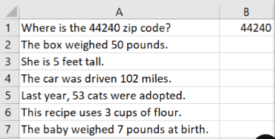
Q148. What feature can you use to populate B2:B7 with the number from each sentence in A2:A7?
- No Excel feature can accomplish this; this is possible only using formulas.
- Flash Fill✔
- Merge cells
- Text to columns
Q149. Which choice causes a circular error when it is included in a worksheet formula?
- a reference to the cell occupied by the formula✔
- a named constant
- a worksheet function
- a defined formula name
Q150. You have a worksheet with the year in column A, the month in column B, and the day in column C. All fields contain numbers. What function would you use to create the date column in D?
- DATEVALUE✔
- CONCATENATE
- TEXTJOIN
- DATE
Q151. You have a column containing runner times for a recent race. What function could you use to find the second-place finisher (the runner with the second-lowest time)?
- SMALL
- MATCH✔
- MIN
- NEXT
Q152. What is the default horizontal alignment of text in a cell
- left✔
- bottom
- top
- right
Q153. Which formula adds 8 and 5 in a cell?
- =ADD(8+5)
- 8+5
- None of these answers, as you cannot add without a
SUMfunction. - =8+5✔
Q154. What feature allows you to make the text appear as it does in cell B1:F1?

- cell border
- merge cells
- text orientation✔
- wrap text
Q155. What type of chart is this?

- histogram✔
- waterfall
- treemap
- box and whisker
Q156. What type of chart is this?
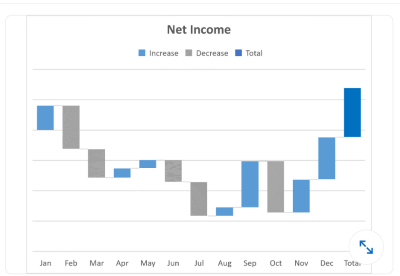
- histogram
- waterfall✔
- treemap
- box and whisker
Q157. How do you override Excel’s automatic axis scaling to enter custom axis maximum and minimum values?
- You cannot do this in Excel.
- Right-click the axis, select Format Axis, and scroll to the desired minimum and maximum values.
- Right-click the axis and select Format Axis > Axis Options. Then change the minimum and maximum values.✔
- Click the individual axis values and change them manually.
Q158. Given the source data, how do you transform the middle PivotTable to appear like the rightmost PivotTable?
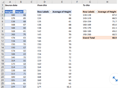
-
­ -
­ - The below answer should be right
- Right-click any row field value in the pivot table and select Group.✔
Q159. Which formula will calculate the number of blank cells in the range A1:A20
- =COUNTBLANK(A1:A20)✔
- =COUNTA(A1:A20)
- =COUNTIF(A1:A20,”>0″)
- =COUNT(A1:A20)
Q160. A mortgage lender requires a 20% down payment and is offering a 30-year loan with a 3.5% interest rate. Which Excel function can you use to calculate the maximum purchase price you can afford?
- Power Query
- NPV✔
- Goal Seek
- Scenario Manager
Q161. You have filtered a table. How can you tell which column a table is sorted by?
- The sorted-by-column heading will be italicized
- The sorted-by-column heading will be bold
- The sorted-by-column heading filter will have an arrow icon✔
- The sorted column will be lightly shaded
Q162. How many users can open an Excel file at the same time?
- 64
- 128
- 256✔
- 512
Q163. How to specify the cell range from A9 to A99 in Excel?
- (A9 ∶ A99)✔
- (A9 – A99)
- (A9 , A99)
- (A9 to A99)